This leads us to a question: do simpler "solutions" exist that would allow a trader to manage the exposure of a position to interest rate risk using fewer securities? In this section, we motivate this by examining interest rate exposure profiles. Visually and numerically, we will see how the value of a bond portfolio changes with shifts in yields. For example, what happens if all yields rise or fall by 1%?

Example 6.3.1

In this example, we will consider the impact of large yield curve shifts. Consider the following securites, which generates cash flows over four years as follows.

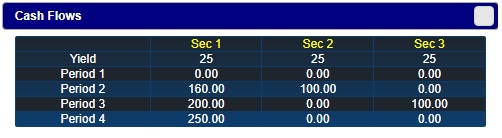
The first security has cash flows in periods 2, 3, and 4. The second is a two-period zero coupon bond. The third is a three-period zero coupon bond. In addition, there is a cash or money-market account that pays 25% interest. The yield on every bond is 25%.

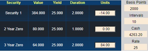
Securities and Units

The starting position is:

• Security 1: -14 units (a short position)
• Security 2: 51 units
• Security 3: 0 units
• Cash: $5,300

Online, you can work with this problem using the interactive online calculator below. If the positions are not initialized, select "Set Position" under Example 6.3.1.

Note:We measure shifts by "basis points." One basis point is equal to 1/100 of a percent, so 100 basis points equals 1%. The calculator below allows you to set the range of basis points and also the number of intervals or shifts ot display. For exam, if you set it to 100 basis points and 10 intervals, you will see the result of yield shifts from -100bp to +100 bp divided into 20 intervals, 10 for positive shifts, 10 for negative shifts.

You can see that this position benefits from an increase in interest rates and is hurt by a decrease.

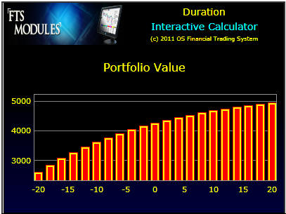
Numerically, the portfolio value for different shifts in yields can be viewed by clicking on the Numeric button:

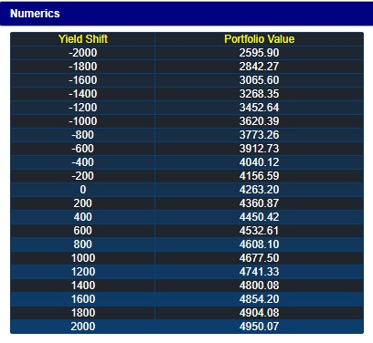
You can see that the present value of the portfolio is exposed to shifts in the yield curve.

With all yields at 25%, the current value of this position is:

-14* $307.2 + 51* $64 + $5,300= $4,263.20

Future Values

In practice, we must consider the effects of a yield curve shift at the end of some period of time. That is, the position is invested at the current spot rate and then during the period the yield curve shifts to a new level. To consider the effects of this scenario, compute the value of this position at the end of the year:

$4,263.20 * 1.25 = $5,329

In the calculator, you can verify this by selecting "Future Value" under Example 6.3.1 or by checking "+1 Year" to see the values at the end of Year 1. Click on the "Numeric" button to see the portfolio values in one year for different shifts in the yield curve.

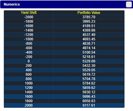
Let us verify one calculation. Suppose the yield curve shifts up during the first year so that at year end it is a flat 35%, i.e. shifts up by 1000 basis points or 10%. This shift reduces the value of both the asset (i.e., the long position) and the liability (i.e., the short position).

Overall, the total value changes as follows. Security 1 is now worth $329.86 = 160/(1.35) + 200/(1.35^2) + 250/(1.35^3). Security 2 is now worth $74.07 = 100/1.35. Security 3 is worth $54.89 = 100/(1.35^2)

$5,300*1.25 -14*329.86 + 51*74.07 = $5,784.62

By calculating the present values for different shifts in the curve, you can verify the other values shown in the Numerics window.

How can you ensure that this position never falls below $5,000 in one year?

An easy solution is to cash out. At the current yield curve this locks you into $5,329, which satisfies your constraint with a little excess to spare. However, at any point in time, a firm's position consists of two types of short (liabilities) and long (assets) positions: those that are held for trading purposes and those that are not intended to be liquidated during the firm's normal course of business over the current period.

Suppose the liability, -14 units of Security I, cannot be traded but you still want to manage the interest rate risk associated with this position. In particular, you want to ensure that by year end its value does not fall below $5,000 over the given range of yield curve shifts.

How can you achieve this?

Consider buying 84 3-year zeroes and selling the position 51 2-year zeroes at todays prices ($64 and $51.2 respectively). Selling the 2-year zeros raises 51*64 = $3,264 while buying 84 3-year zeros costs $4,300.80, so you cash gets reduced from $5,300 to $4,263.20. In the calculator, select "Future Value" under Example 6.3.2.

Online, a very different picture emerges. The values of this position in one year for different yield curve shifts is:

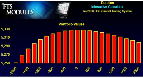
You can see the numbers underlying the chart by clicking the "Numeric" button as before.

Both the numeric values and the chart show that our position stays above $5000 at year end, for a wide range of yield curve fluctuations! That is, your position is hedged against fluctuations in the yield curve.

In summary to hedge this position recall that you engaged in the following transactions at the beginning of the year:

i. Sold 51 units of Security 3 at $64 (the present value of $100 at the end of Year 2 using the spot flat 25% yield curve). This equals $3,264 (51*$64).

ii. Bought 84 units of Security 4 at $51.20 (the present value of $100 at the end of Year 3 using the spot flat 25% yield curve). This equals $4,300.80 (84*$51.20).

iii. Invested the remaining balance of cash in the money market at 25%. This equals $4,263.20*1.25 ($5,300 + $3,264 - $4,300.80 = $4,263.20).

Numerically, the year-end value of this position, if there is no shift in the yield curve, equals:

$4,263.20 * 1.25 - 14 * $384 + 84 * $64 = $5,329

Yield Curve at end of Year 1: Value of Position

(1, 2, and 3 year spot rate) at End of Year 1

5%, 5%, 5% $5251.60 (= $5,329 - $77.40)

15%,15%,15% $5314.27 (= $5,329 - $14.73)

25%,25%,25% $5329

35%,35%,35% $5319.90 (= $5,329 - $9.10)

45%,45%,45% $5299.61 (= $5,299.61 - $29.39)

You can see that this new position satisfies the $5,000 constraint over a range of 2,000 basis points shift in the yield curve.

In this trading approach to hedging interest rate risk be sure to distinguish between the time of adjusting the position (the beginning of the year) with the time for which protection is desired (at the end of the year).

In the calculator, you may have noticed a number called Duration shown just below the securities. In the next section, we will explain what this is, and an important result called the bond immunization theorem. After develop this theory in the next topic, Macaulay's Duration, we will return to this example in section 6.5 to see how it can be used to hedge interest rate risk.